Quantum error mitigation by layerwise Richardson extrapolation
In a previous post, I gave a high-level overview of zero-noise extrapolation (ZNE) and how we can increase the noise of quantum circuits for ZNE using a technique known as quantum circuit unoptimization. In this post, I’ll describe a technique that my colleague Andrea Mari and I came up with called layerwise Richardson extrapolation (LRE), which can be thought of as a generalization of standard ZNE.
The paper can be found on arXiv (arXiv:2402.04000) and was published in Physical Review A (Phys. Rev. A 110, 062420, 2024). LRE has also been integrated into the open-source quantum error mitigation toolkit mitiq, developed by the Unitary Foundation.
Quick recap: standard ZNE#
To set the stage, let’s briefly recap how standard ZNE works (see the previous post for more detail). The idea is:
- Take a quantum circuit and create multiple copies of it where the noise has been progressively amplified (e.g., via unitary folding).
- Execute each noisy circuit and collect the expectation values.
- Fit a curve through these data points and extrapolate back to the zero-noise limit.
The key point is that standard ZNE treats the circuit’s noise as a single scalar parameter \(\lambda\). When you fold the circuit (say, with global folding), every layer gets scaled by the same factor. The extrapolation is then a univariate polynomial fit: \(f(\lambda) = a_0 + a_1\lambda + a_2\lambda^2 + \cdots\).
This is a perfectly reasonable approach, but it makes an implicit assumption: that all layers of the circuit experience the same type and magnitude of noise. In practice, this is often not the case. Different layers can have different gate error rates, different qubit connectivities, and different levels of crosstalk. Standard ZNE has no way to account for this layer-to-layer variation.
The idea behind LRE#
The core idea of LRE is to treat the noise in each circuit layer as an independent variable. Instead of a single noise-scale factor \(\lambda\), we now have a vector of scale factors \(\mathbf{\lambda} = (\lambda_1, \lambda_2, \ldots, \lambda_l)\), where \(l\) is the number of layers in the circuit.

By scaling each layer independently, we can capture the distinct noise characteristics of different parts of the circuit. The extrapolation then becomes a multivariate polynomial fit over this higher-dimensional space, allowing for a more fine-grained and accurate estimate of the zero-noise expectation value.
How LRE works#
The LRE workflow consists of two main stages:

Stage 1: Multivariate noise scaling. Given a circuit with \(l\) layers and a chosen polynomial degree \(d\), we generate a collection of noise-scaled circuits. Each circuit in this collection has its layers folded according to a specific scale-factor vector \(\mathbf{\lambda}_i = (\lambda_1^{(i)}, \lambda_2^{(i)}, \ldots, \lambda_l^{(i)})\). The total number of noise-scaled circuits we need is determined by the number of monomials in the multivariate polynomial basis:
$$M = \binom{d + l}{d}$$For example, with degree \(d = 2\) and \(l = 2\) layers, the monomial basis is \(\{1, \lambda_1, \lambda_2, \lambda_1^2, \lambda_1\lambda_2, \lambda_2^2\}\), giving us \(M = 6\) terms and hence 6 noise-scaled circuits.
Stage 2: Multivariate Richardson extrapolation. After executing all the noise-scaled circuits and collecting their expectation values \(\langle O(\mathbf{\lambda}_i)\rangle\), we compute the zero-noise estimate as a linear combination:
$$O_{\text{LRE}} = \sum_{i=1}^{M} c_i \langle O(\mathbf{\lambda}_i)\rangle$$The coefficients \(c_i\) are determined analytically from multivariate Lagrange interpolation theory. Specifically, they are given by the ratio of determinants:
$$c_i = \frac{\det(B_i(\mathbf{0}))}{\det(A)}$$where \(A\) is the sample matrix formed by evaluating the monomial basis at each scale-factor vector, and \(B_i(\mathbf{0})\) is the matrix obtained by replacing the \(i\)-th row of \(A\) with the monomials evaluated at \(\mathbf{\lambda} = \mathbf{0}\) (i.e., the zero-noise point). This is analogous to Cramer’s rule applied to the interpolation problem.
Using LRE in mitiq#
LRE is available in mitiq, making it straightforward to apply in practice. Here’s a minimal example using Cirq:
import numpy as np
from cirq import (
    DensityMatrixSimulator, depolarize,
    LineQubit, Circuit, Moment,
    H, CNOT, rx, ry,
)
from mitiq.lre import execute_with_lre

# Define a circuit with a few layers.
qubits = LineQubit.range(2)
circuit = Circuit([
    Moment([H(qubits[0])]),
    Moment([CNOT(qubits[0], qubits[1])]),
    Moment([rx(np.pi / 4).on(qubits[0]), ry(np.pi / 3).on(qubits[1])]),
])

# Define an executor that simulates a noisy backend.
def execute(circuit, noise_level=0.02):
    noisy_circuit = circuit.with_noise(depolarize(p=noise_level))
    rho = DensityMatrixSimulator().simulate(noisy_circuit).final_density_matrix
    return np.real(rho[0, 0])

# Run LRE.
mitigated_value = execute_with_lre(
    circuit,
    execute,
    degree=2,
    fold_multiplier=3,
)

noisy_value = execute(circuit)
ideal_value = execute(circuit, noise_level=0.0)

print(f"Ideal value:     {ideal_value:.5f}")
print(f"Noisy value:     {noisy_value:.5f}")
print(f"Mitigated (LRE): {mitigated_value:.5f}")
Running this produces:
Ideal value:     0.33839
Noisy value:     0.32722
Mitigated (LRE): 0.33687
The LRE-mitigated value (0.33687) is closer to the ideal (0.33839) than the raw noisy value (0.32722), reducing the error from ~0.011 to ~0.002. The two key parameters are:
degree: The degree of the extrapolating polynomial. Higher degree can capture more complex noise behavior, but requires more noise-scaled circuits.fold_multiplier: Controls how aggressively each layer is folded. A larger fold multiplier means more separation between noise levels.
Under the hood#
If you want more control, mitiq exposes the two stages of LRE as separate functions:
from mitiq.lre.multivariate_scaling import multivariate_layer_scaling
from mitiq.lre.inference import multivariate_richardson_coefficients

# Stage 1: Generate noise-scaled circuits.
noise_scaled_circuits = multivariate_layer_scaling(circuit, degree=2, fold_multiplier=3)
print(f"Number of noise-scaled circuits: {len(noise_scaled_circuits)}")

# Execute each noise-scaled circuit.
noisy_exp_values = [execute(circ) for circ in noise_scaled_circuits]

# Stage 2: Compute Richardson coefficients and combine.
coefficients = multivariate_richardson_coefficients(
    circuit, fold_multiplier=3, degree=2
)

mitigated_value = sum(
    exp_val * coeff for exp_val, coeff in zip(noisy_exp_values, coefficients)
)
Number of noise-scaled circuits: 10
Mitigated (manual): 0.33687
For this 3-layer circuit with degree 2, we need \(\binom{2+3}{2} = 10\) noise-scaled circuits. This gives you the flexibility to batch the circuit executions, use different backends, or inspect the intermediate noise-scaled circuits.
Performance comparison: LRE vs. ZNE#
To see how LRE compares to standard ZNE, consider a 12-moment circuit under layer-dependent noise where later layers experience up to 5x higher depolarizing rates than early layers:

Averaging over 10 random circuits at each noise level, LRE consistently achieves lower error than ZNE:
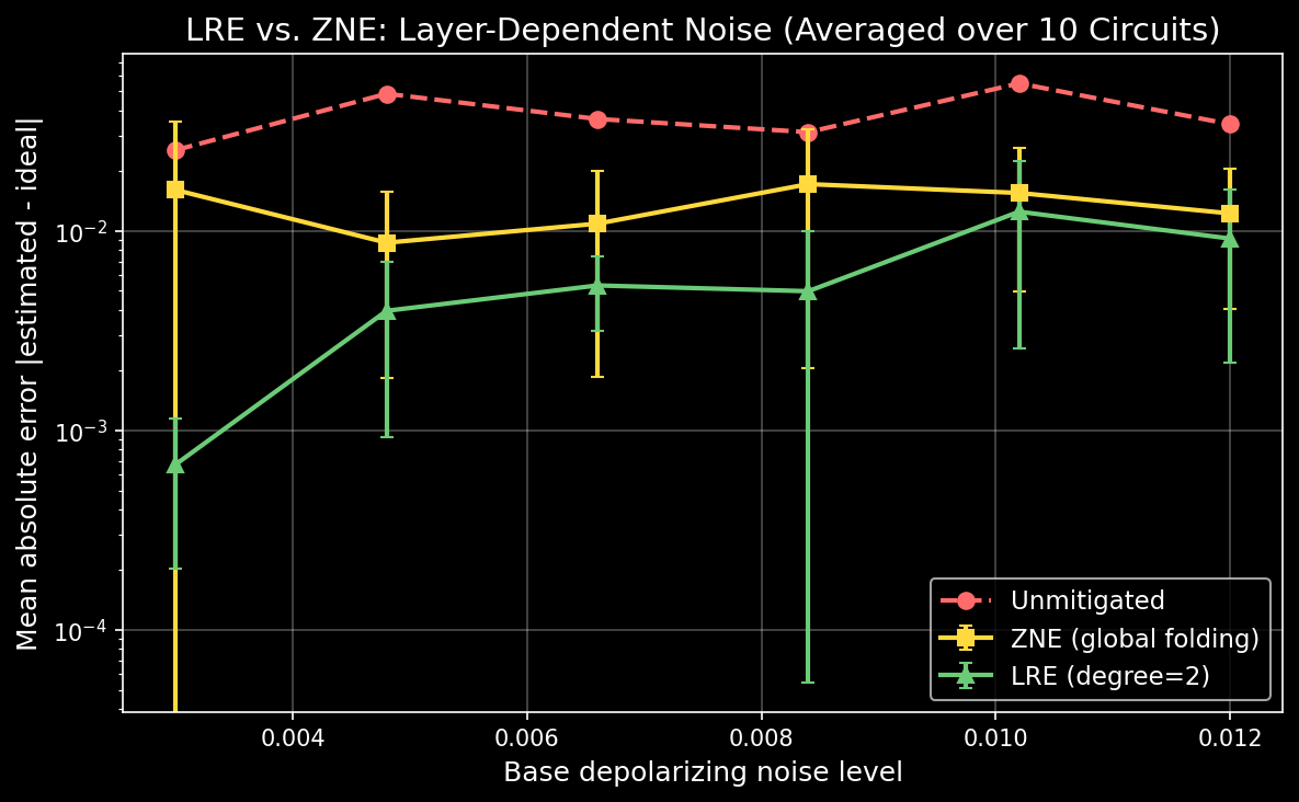
The trade-off is circuit overhead: for a 12-layer circuit with degree 2, LRE requires \(\binom{14}{2} = 91\) noise-scaled circuits, while ZNE typically uses 3-5. Whether this is worthwhile depends on your application—on simulators the overhead is negligible, while on real hardware with limited shot budgets, chunking (discussed below) can reduce the number of circuits substantially.
The benefit is most pronounced for deeper circuits where noise accumulation across layers becomes significant. For shallow circuits or uniform noise, LRE and ZNE tend to perform similarly (since uniform noise reduces the multivariate model to the univariate case).
Tuning LRE: degree and fold multiplier#
The two main hyperparameters that control LRE’s behavior are the polynomial degree and the fold multiplier. Higher degree allows the polynomial to capture more complex noise dependencies, but requires exponentially more noise-scaled circuits. The fold multiplier controls the spacing between noise levels.
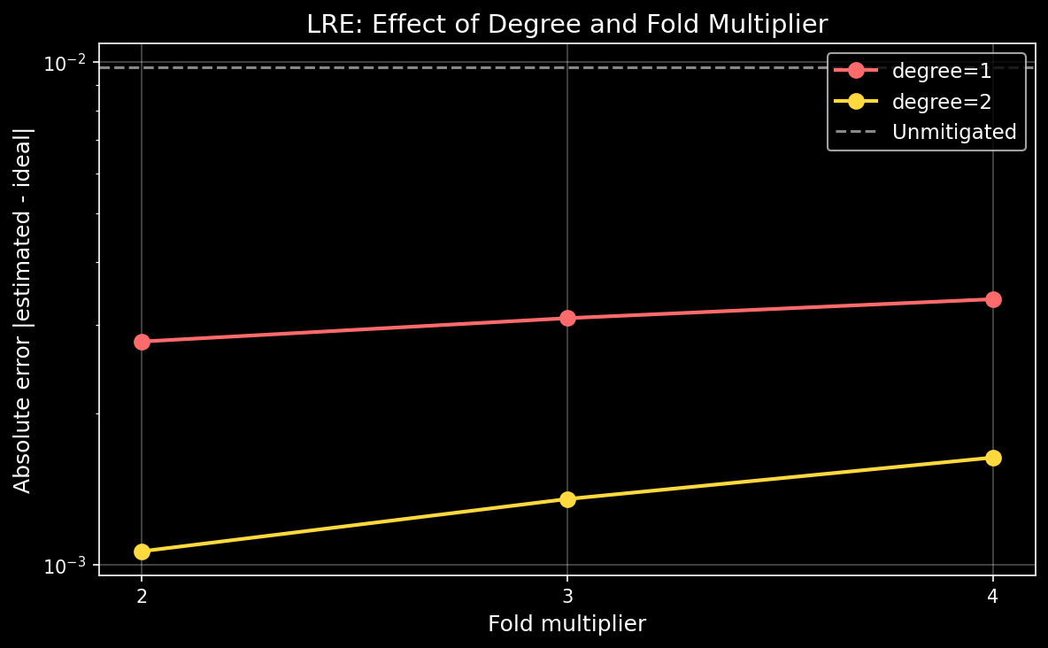
As the plot shows, increasing the degree from 1 to 2 yields lower error, as the polynomial model becomes more expressive. Degree 3 is not shown because the sample matrix becomes too large to compute determinants reliably even for an 8-layer test circuit—this is exactly where chunking becomes necessary.
Chunking: handling large circuits#
For circuits with many layers, the number of required noise-scaled circuits grows combinatorially. The formula \(M = \binom{d+l}{d}\) means that a 20-layer circuit at degree 2 requires 231 noise-scaled circuits, and a 20-layer circuit at degree 3 requires 1771.
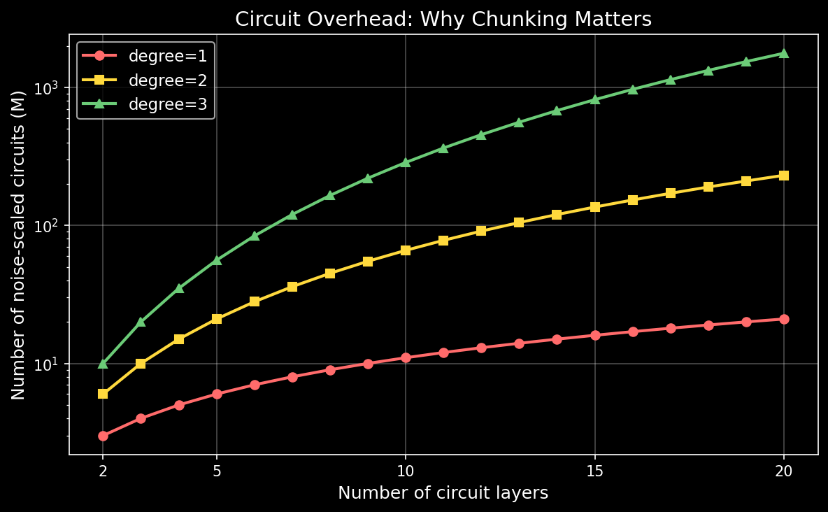
To address this, LRE supports chunking, where consecutive layers are grouped together and treated as a single unit for the purposes of noise scaling. This reduces the effective number of independent variables from \(l\) to the number of chunks.
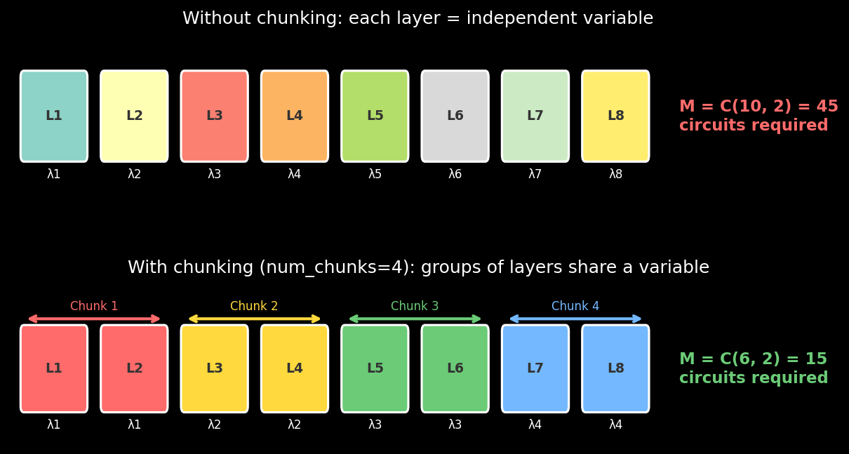
The visualization above shows how an 8-layer circuit, which would require \(\binom{10}{2} = 45\) noise-scaled circuits without chunking, only requires \(\binom{6}{2} = 15\) circuits when grouped into 4 chunks. In mitiq, this is a single parameter:
mitigated_value = execute_with_lre(
    circuit,
    execute,
    degree=2,
    fold_multiplier=3,
    num_chunks=4,  # Group layers into 4 chunks.
)
This trades some granularity in the layer-by-layer noise model for practical feasibility. For large circuits, chunking is essential to keep the circuit overhead manageable.
When to use LRE#
LRE is particularly well-suited for circuits where different layers have meaningfully different noise characteristics. This includes scenarios where:
- The circuit has a mix of single-qubit and two-qubit gate layers (two-qubit gates typically have higher error rates).
- The circuit uses qubits with varying coherence times or gate fidelities.
- Crosstalk effects are localized to specific layers.
- Noise accumulates with circuit depth (as is common on real hardware).
When the noise is perfectly uniform across all layers, LRE and standard ZNE yield similar results (as expected, since uniform noise means the multivariate model degenerates to the univariate case). So there is no penalty for using LRE in the uniform case—it simply reduces to the standard approach.
Further reading#
- Paper: arXiv:2402.04000 (Phys. Rev. A 110, 062420, 2024)
- Mitiq docs: LRE user guide