Digital zero-noise extrapolation via quantum circuit unoptimization
While quantum computers have continued to improve over the past few years, it’s a known issue that error rates cannot be made low enough simply by improvements to the hardware. One approach to this problem is the domain of quantum error correction (QEC) which promises fault-tolerant devices that properly deals with the issue of noise. While the theory of QEC is well-established, the implementation of the theory is still a while away from being physically realizable. One strategy to deal with the noise in a less idealized manner in the interim is the field of quantum error mitigation (QEM).
There are a variety of QEM techniques that are the subject of active research, for example, zero-noise extrapolation (ZNE), probabilistic-error cancellation (PEC), dynamical decoupling (DD), and Clifford data regression (CDR) to name a few.
Zero-noise extrapolation (ZNE)#
As you can probably tell from the title, we will be focused on ZNE in this post. The general idea of ZNE is quite simple (although, perhaps at first, a bit counterintuitive). Here’s a memorable tongue-and-cheek description of the technique:
Basic idea of ZNE: Quantum computers are noisy and they kinda suck. To make them suck less you can do something counterintuitive and deliberately make them suck even more by chopping up the quantum circuit you want to run on the quantum computer and increasing the suck factor. Then, you can statistically extrapolate the suckiness of how much it sucked to the point of least suckiness.
Let’s make this a bit more formal. You have a quantum circuit that you want to run on a quantum computer. You know that the device is inherently noisy, so you expect your result to be impacted by this noise. However, you would like to know what the output of your computation was if you had run it in an ideal (noiseless) environment.
Progressively increase the noise for a set of quantum circuits that are obtained from your original quantum circuit (we will discuss ways to do this later). Generate a set of data points by calculating expectation values for each circuit in this set.
Plot each of these expectation values on a graph and draw a line through them (extrapolate) to the so-called “zero-noise limit” to infer what the expectation would be if it was executed in a noiseless environment.
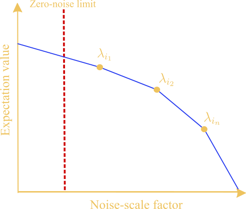
That’s the basic idea in a nutshell; pump up the volume and then ride the wave. The figure above shows the basic idea of how these two steps can be used to statistically infer the expectation value at the zero-noise limit. Each of the data points labeled as \(\lambda_{i_1}, \lambda_{i_2}\), and \(\lambda_{i_n}\) are called noise-scale factors (which we describe in greater detail in the subsequent sections).
Boosting the volume (increasing the noise)#
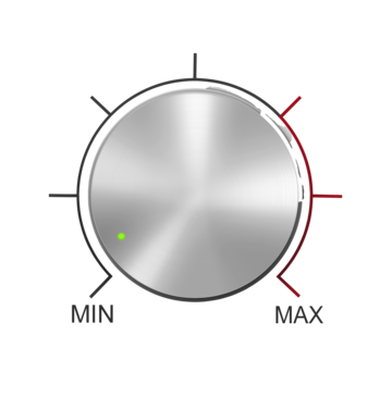
So how can one increase the noise of a quantum circuit, and do so in a way that is controlled. It’s not difficult to completely garble the circuit so that it’s a complete mess of noise and sadness (which is not helpful for us). Instead, we want something like a volume knob that, at specific discrete points in the dial, turns the volume up by a specific amount.
One way you can do this for quantum circuits (like the ones you might define in a library like Qiskit to be run on a quantum computer) would be to use the technique of unitary folding. Given a quantum circuit, unitary folding increases the effective length (or depth) of the quantum circuit by adding a larger number of gates in a specific way which inherently increases the noise.
There are a couple of different flavors of unitary folding, but for simplicity we will just look at global folding. The other folding techniques are all means to the same end with minor tweaks, but global folding is one of the more straightforward approaches.
In global folding each set of layers in the circuit are replaced by \(G G^{\dagger}G\). Since \(G G^{\dagger} = \mathbb{I}\), in the case where we are running our circuit on an ideal (noiseless) simulator this has no effect on the circuit. However, if we run this circuit on a noisy device, this increases the noise and effective gate errors of the computation.
The “volume level” (or noise-scale factor) is usually referred to as a parameter \(\lambda\), which in this case, determines how many times to fold the gates in the circuit.

An example of the global folding technique applied to an arbitrary quantum circuit can be seen in the above figure. For a given collection of gates denotes by \(G\), we increase the effective length of the overall circuit by create \(G G^{\dagger} G\).
Quantum circuit unoptimization#
In a nutshell, quantum circuit unoptimization is a procedure applied to a quantum circuit that makes it more complicated by increasing the depth and gates of the circuit, but keeping the overall output of the circuit the same. That is, if you run something through the original circuit and run the same thing through the unoptimized circuit, the result in both cases will be unitarily equivalent.
Why would anyone want to do this—aren’t people are concerned with optimizing a quantum circuit? Well, yes, usually this is the case. However, one primary reason to do this is to check how good quantum hardware compilers are at simplifying garbled circuits.
In our instance, we are interested in techniques that can effectively increase the noise of a quantum circuit in a deliberate and controlled manner. Quantum circuit unoptimization gives us one way of doing that.
So what is the process of unoptimizing a quantum circuit? Well, as described by the authors in arXiv:2311.03805, it can be done by following a specific recipe that consists of four steps, namely:
Insert: Insert a two-qubit gate \(A\) and its Hermitian conjugate \(A^{\dagger}\) between two gates in the circuit labeled as \(B_1\) and \(B_2\).
Swap: Swap the \(B_1\) gate with the \(A^{\dagger}\) gate in the circuit, replacing \(A^{\dagger}\) with \(\widetilde{A^\dagger}\).
Decompose: Decompose multi-qubit unitary gates into elementary gates.
Synthesize: Apply quantum circuit synthesis.
For a given quantum circuit, you apply the four steps of the recipe. At the end, the quantum circuit cake that you’ve baked is a much more complicated quantum circuit. You can apply this recipe as many times as you like. Each time you do so, the circuit will end up being longer and more complicated. Importantly, however, the output of the final circuit remains unitarily equivalent to the output of the initial circuit.
We implemented this process in Python using Qiskit quantum circuits and released this as companion software for our paper (GitHub). As an example, consider the following arbitrary quantum circuit:
from qiskit import QuantumCircuit

# Create a 4-qubit fully connected graph state.
num_qubits = 4
qc = QuantumCircuit(num_qubits)

for qubit in range(num_qubits):
    qc.h(qubit)

for i in range(num_qubits):
    for j in range(i + 1, num_qubits):
        qc.cz(i, j)
This is just an arbitrary circuit consisting of one and two-qubit gates that in this case represents a 4-qubit fully connected graph state (for the sake of example).
>>> print(qc)
     ┌───┐
q_0: ┤ H ├─■──■──■──────────
     ├───┤ │  │  │
q_1: ┤ H ├─■──┼──┼──■──■────
     ├───┤    │  │  │  │
q_2: ┤ H ├────■──┼──■──┼──■─
     ├───┤       │     │  │
q_3: ┤ H ├───────■─────■──■─
     └───┘
We can use the unoptimize_circuit function from our software package on this circuit and apply as many rounds of the
unoptimization recipe as we would like. For the sake of not giving you carpal tunnel syndrome from having to scroll
such a large circuit, let’s just apply a single iteration of the recipe.
>>> from unopt.recipe import unoptimize_circuit
>>> unoptimize_circuit(qc, iterations=1)
global phase: 2.0949
     ┌────────────────────────┐           ┌────────────────┐          ┌──────────────────────────┐                            ┌──────────────────────────┐     »
q_0: ┤ U3(2.0356,π/2,-2.1618) ├──■────────┤ U3(π,-π/4,π/4) ├───────■──┤ U3(1.2421,-1.84,-1.2786) ├──■──────────────────────■──┤ U3(0.83219,-π/2,-0.5782) ├──■──»
     └──┬──────────────────┬──┘┌─┴─┐┌─────┴────────────────┴────┐┌─┴─┐├──────────────────────────┤  │                      │  └──────────────────────────┘┌─┴─┐»
q_1: ───┤ U3(2.1322,π/2,0) ├───┤ X ├┤ U3(1.7549,2.0217,-2.3363) ├┤ X ├┤ U3(1.1386,1.7574,1.3842) ├──┼──────────────────────┼──────────────────────────────┤ X ├»
      ┌─┴──────────────────┴┐  └───┘└───────────────────────────┘└───┘└──────────────────────────┘┌─┴─┐┌────────────────┐┌─┴─┐    ┌──────────────────┐    └───┘»
q_2: ─┤ U3(π/2,0.062179,-π) ├─────────────────────────────────────────────────────────────────────┤ X ├┤ U3(0,0,1.0704) ├┤ X ├────┤ U3(0.68791,-π,0) ├─────────»
      └─────────────────────┘                                                                     └───┘└────────────────┘└───┘    └──────────────────┘         »
q_3: ──────────────────────────────────────────────────────────────────────────────────────────────────────────────────────────────────────────────────────────»
                                                                                                                                                               »
«           ┌───────────────┐              ┌────────────────────┐                                               ┌───────────────┐                ┌──────────────────────┐          »
«q_0: ──────┤ U3(π/2,0,π/2) ├────────■─────┤ U3(3.0151,-π,-π/2) ├──────────────────────────────────────■────────┤ U3(π/2,0,π/2) ├────────■───────┤ U3(1.132,-0.51688,0) ├───────■──»
«     ┌─────┴───────────────┴─────┐┌─┴─┐┌──┴────────────────────┴─┐     ┌───────────────────────────┐┌─┴─┐┌─────┴───────────────┴─────┐┌─┴─┐┌────┴──────────────────────┴────┐  │  »
«q_1: ┤ U3(2.0383,2.2097,-2.8185) ├┤ X ├┤ U3(1.5857,-0.9553,-π/2) ├──■──┤ U3(0.56249,-π/2,-0.81816) ├┤ X ├┤ U3(2.0383,2.2097,-2.8185) ├┤ X ├┤ U3(0.039343,0.031289,0.031289) ├──┼──»
«     └───────────────────────────┘└───┘└─────────────────────────┘┌─┴─┐└─┬───────────────────────┬─┘└───┘└───────────────────────────┘└───┘└────────────────────────────────┘┌─┴─┐»
«q_2: ─────────────────────────────────────────────────────────────┤ X ├──┤ U3(1.0967,0.40856,-π) ├───────────────────────────────────────────────────────────────────────────┤ X ├»
«                                                                  └───┘  └───────────────────────┘                                                                           └───┘»
«q_3: ─────────────────────────────────────────────────────────────────────────────────────────────────────────────────────────────────────────────────────────────────────────────»
«                                                                                                                                                                                  »
«                             ┌─────────────────────────┐            ┌────────────────┐          ┌─────────────────────────────┐      ┌───────────────────────┐       »
«q_0: ─────────────────────■──┤ U3(π,-0.51538,-0.51538) ├───■────────┤ U3(π,-π/4,π/4) ├───────■──┤ U3(2.2152,-0.15561,-1.6024) ├──■───┤ U3(0.40369,-π/2,-π/2) ├────■──»
«                          │  └─────────────────────────┘ ┌─┴─┐┌─────┴────────────────┴────┐┌─┴─┐└───┬─────────────────────┬───┘  │   └───────────────────────┘    │  »
«q_1: ─────────────────────┼──────────────────────────────┤ X ├┤ U3(1.7231,1.9856,-2.2664) ├┤ X ├────┤ U3(2.1322,-π/2,π/2) ├──────┼────────────────────────────────┼──»
«     ┌─────────────────┐┌─┴─┐┌──────────────────────────┐└───┘└───────────────────────────┘└───┘    └─────────────────────┘    ┌─┴─┐┌──────────────────────────┐┌─┴─┐»
«q_2: ┤ U3(0,0,-1.3608) ├┤ X ├┤ U3(1.8527,1.8089,1.6118) ├──────────────────────────────────────────────────────────────────────┤ X ├┤ U3(2.1223,3.0309,1.3617) ├┤ X ├»
«     └─────────────────┘└───┘└──────────────────────────┘                                                                      └───┘└──────────────────────────┘└───┘»
«q_3: ────────────────────────────────────────────────────────────────────────────────────────────────────────────────────────────────────────────────────────────────»
«                                                                                                                                                                     »
«         ┌────────────────────┐         ┌──────────────────────────────┐
«q_0: ────┤ U3(0.29827,0,-π/2) ├──────■──┤ U3(1.9596,-0.96632,-0.54303) ├───────■──────────────────────────────────────────
«         └────────────────────┘      │  └──────────────────────────────┘       │
«q_1: ────────────────────────────────┼────────────────────────────────────■────┼───────────────────■──────────────────────
«     ┌────────────────────────────┐┌─┴─┐┌─────────────────────────────┐ ┌─┴─┐  │  ┌─────────────┐  │
«q_2: ┤ U3(1.1033,0.32306,-2.2097) ├┤ X ├┤ U3(0.23528,0.096677,2.2331) ├─┤ X ├──┼──┤ U3(π/2,0,π) ├──┼────■─────────────────
«     └────────────────────────────┘└───┘└─────────────────────────────┘ └───┘┌─┴─┐└─────────────┘┌─┴─┐┌─┴─┐┌─────────────┐
«q_3: ────────────────────────────────────────────────────────────────────────┤ X ├───────────────┤ X ├┤ X ├┤ U3(π/2,0,π) ├
«                                                                             └───┘               └───┘└───┘└─────────────┘
From a cursory visual inspection, this circuit looks wildly different than the original one. The more iterations you subsequently apply, the larger and more garbled the circuit will become. However, it will remain unitarily equivalent to the original circuit (even if it looks quite a bit different). You can confirm this by doing a sanity check:
from qiskit.quantum_info import Operator

unopt_qc = unoptimize_circuit(qc, iterations=1)

original_unitary = Operator(qc)
unopt_unitary = Operator(unopt_qc)

unitaries_are_equal = original_unitary.equiv(unopt_unitary)
Indeed, we can see that the original and unoptimized circuit are unitarily equivalent:
>>> print(f"Are the circuits functionally equivalent? {unitaries_are_equal}")
Are the circuits functionally equivalent? True
You can continually bump up the number of iterations, and the circuits will remain unitarily equivalent.
Unoptimization and ZNE#
Like unitary folding, we can use the technique of circuit unoptimization to progressively increase the noise and extrapolate to the zero-noise limit. In our paper, (arXiv:2503.06341), we considered this on two classes of circuits that people find interesting for various reasons; quantum volume (QV) and Quantum Approximate Optimization Algorithm (QAOA) circuits.
I’ll leave the detailed analyses of how quantum circuit unoptimization can be used for those classes of circuits to the paper. However, we can take a more general look at how one can apply unoptimization as a noise-scaling technique for ZNE. Furthermore, we can also compare how this noise-scaling does in comparison to the ideal (noiseless) case, the unmitigated case (i.e. running the circuit in a noisy setting with no error mitigation), and the case where ZNE is used but some type of unitary folding is applied for the noise-scaling.
We can perform comparative benchmarks for ZNE with unoptimization as a scaling technique against the ideal, unmitigated, and ZNE with folding
>>> from unopt.benchmark import bench
Averages Across All Trials:
  Ideal Value: 0.06250000000000006
  Unmitigated Value: 0.003799999999999956
  ZNE + Fold Value: 0.00037500000000005443 (Error: 0.062125)
  ZNE + Unopt Value: 0.008441716269841373 (Error: 0.05405828373015868)
  Percent Improvement (Unmit): 8.59%
  Percent Improvement (ZNE + Fold): 14.92%
  Original Circuit Depth: 6
  Avg Folded Depths: [6.0, 18.0, 30.0]
  Avg Unoptimized Depths: [37.0, 65.0, 101.0]


Trial Details:
Trial 1:
  Ideal Value: 0.06250000000000006
  Unmitigated Value: 0.003799999999999956
  ZNE + Fold Value: 0.00037500000000005443
  ZNE + Fold Depths: [6, 18, 30]
  ZNE + Unopt Value: 0.008441716269841373
  ZNE + Unopt Depths: [37, 65, 101]
Note that for certain circuits and runs, you may obtain different results as there is a randomized component to the circuit unoptimization and extrapolation.
Further reading#
This post is just a high-level overview of the ideas elaborated on in more detail in the paper, so for further information, examples, etc., please check out both the arXiv preprint (arXiv:2503.06341) as well as the software (GitHub).