Compressed sensing for efficient fidelity estimation of GHZ states
IEEE International Conference on Quantum Computing and Engineering (QCE26)
Farrokh Labib1, David Nicholaeff2,
Vincent Russo1,4,
William J. Zeng1,3
1Unitary Foundation
2New Mexico Consortium
3Quantonation
4IonQ
arXiv:2604.27824
 paper
paper
GHZ states as a hardware benchmark
\[ |\mathrm{GHZ}\rangle = \frac{1}{\sqrt{2}} \bigl(|0\rangle^{\otimes N} + |1\rangle^{\otimes N}\bigr) \]
secret sharing metrology error correction
Fidelity \(F\): how close the built state is to the intended one, from 0 to 1.
(IBM, 2025; \(F > 0.5\))1
to zero
This talk: verify GHZ states with \(\log N\) measurement
circuits instead of \(2N\),
and detect errors during preparation on trapped-ion hardware.
1Javadi-Abhari, Ali, et al. “Big cats: entanglement in 120 qubits and beyond.” arXiv:2510.09520 (2025).
Fidelity as population and coherence
\[ F(\rho) = \langle \mathrm{GHZ} | \rho | \mathrm{GHZ} \rangle = \frac{1}{2}\Bigl( \underbrace{\langle\mathbf{0}|\rho|\mathbf{0}\rangle + \langle\mathbf{1}|\rho|\mathbf{1}\rangle}_{ \text{population } P} + \underbrace{\langle\mathbf{0}|\rho|\mathbf{1}\rangle + \langle\mathbf{1}|\rho|\mathbf{0}\rangle}_{ \text{coherence}} \Bigr) \]
| 0.5 | 0 | 0 | 0.5 |
| 0 | 0 | 0 | 0 |
| 0 | 0 | 0 | 0 |
| 0.5 | 0 | 0 | 0.5 |
| 0.5 | 0 | 0 | 0 |
| 0 | 0 | 0 | 0 |
| 0 | 0 | 0 | 0 |
| 0 | 0 | 0 | 0.5 |
| 0.5 | 0 | 0 | 0.3 |
| 0 | 0 | 0 | 0 |
| 0 | 0 | 0 | 0 |
| 0.3 | 0 | 0 | 0.5 |
Here \(\mathbf{0} = 0\cdots0\) and \(\mathbf{1} = 1\cdots1\). Diagonal entries are outcome probabilities; the corner off-diagonals measure the superposition itself.
A coin flip scores exactly \(F = 1/2\). Everything above \(1/2\) lives in the orange corners: the coherence is the number to measure.
Measuring population and coherence
Average parity follows \(\mathcal{P}(\phi) = C\cos(N\phi + \theta)\); the amplitude \(C \ge 0\) and phase \(\theta\) give \(F(\rho) = (P + C\cos\theta)/2\).
\(Z\) counts cannot see the off-diagonals; after the rotation the coherence shows up as an even/odd bias in the outcomes.
Resolving any frequency blind takes \(2N\) angles1,2: 201 circuits in all at \(N = 100\).
1Nyquist,
“Certain topics in telegraph transmission theory,”
Trans. AIEE 47.2 (1928).
2Shannon,
“Communication in the presence of noise,” Proc. IRE
37.1 (1949).
The parity signal is sparse
- Ideal GHZ parity is a single cosine at frequency \(N\).
- Its recipe, the bottom panel, is zero at every other frequency.
- Real data is noisy, but still approximately sparse.
- Compressed sensing exploits that sparsity: far fewer than \(2N\) samples.
Compressed slide on compressed sensing
- The right-hand chart is the signal's recipe: the signal rewritten as a sum of simple waves, one entry per wave saying how much of it the signal contains. Natural signals have nearly empty recipes.
- A JPEG keeps the few big entries and looks identical, but it measures everything first: fine when a measurement is a cheap pixel.
- Compressed sensing pays for the information rather than the signal length: few random samples, solve for the big entries.1 Ours is the expensive case: each measurement is a quantum circuit.
1Brunton, Steven L., and J. Nathan Kutz. Data-Driven Science and Engineering. Cambridge University Press, 2019.
Random sampling avoids aliasing
Frequency 2, sampled at 8 equally spaced angles.
- Frequency 10 passes through every one of the same samples: \(\cos(10\phi_k) = \cos(2\phi_k)\) exactly. A regular grid has a period for impostors to hide behind; ruling that out for every frequency up to \(N\) is what costs \(2N\).
- A random angle has no period: distinct frequencies agree there with probability zero, so each further sample rules out a roughly constant fraction of the wrong candidates: ∼log(candidates) samples leave one survivor.
Recovery pipeline via compressed sensing
- Lasso for which frequencies, least squares for how big: the penalty that isolates the frequency also shrinks its amplitude, so the refit is unpenalized.
- The Lasso1 fits all candidate frequencies together, with an \(L_1\) penalty; weak candidates are driven exactly to zero.
- Why so few: amplitude and phase absorb the first samples, then each further one rules out a constant fraction of the wrong frequencies, so \(M \propto \log N\) suffices.
1Tibshirani, Robert. “Regression shrinkage and selection via the lasso.” Journal of the Royal Statistical Society B 58.1 (1996).
Choosing the measurement budget
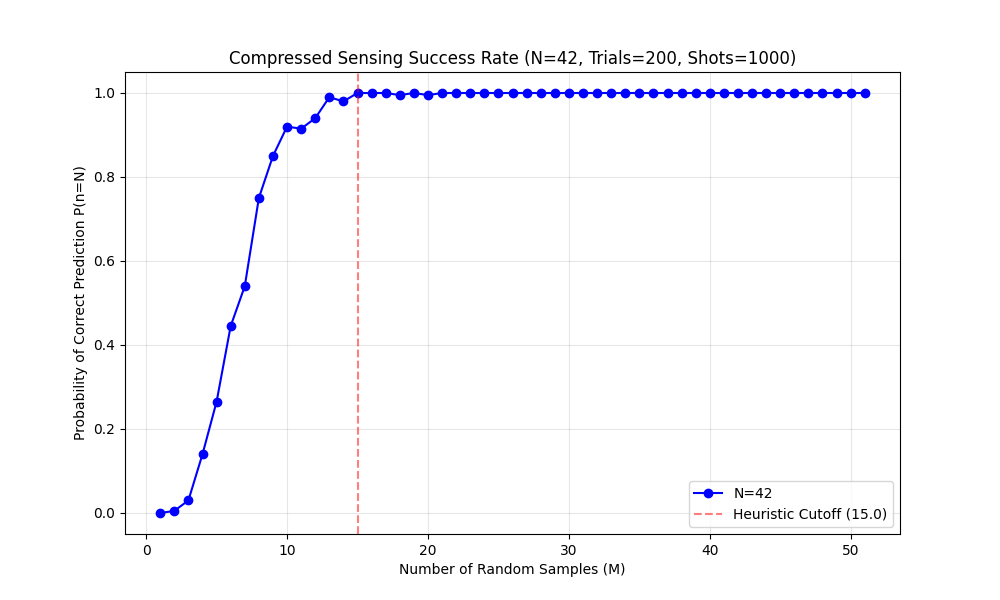
- Recovery improves rapidly with \(M\), then saturates around \(M \approx 15\) for \(N = 42\).
- Choose enough random angles to reach the recovery plateau; beyond that, additional angles give diminishing returns.
- The required budget scales as \(M = O(\log N)\); our rule \(M \approx 5\ln N\) gives 19 angles at \(N = 50\).
Preparing states worth verifying
Preparing a GHZ state: chain versus tree
- Same state, same gate count: only the CNOT schedule differs; every layer is an opportunity for noise, so shallower wins.
- Shallow preparation trades depth for high-weight errors.
How one bit flip spreads
- A CNOT copies bit flips:
- \(\mathrm{CNOT}(X \otimes I) = (X \otimes X)\mathrm{CNOT}\).
- Damage depends on when the fault happens rather than how big it is.
- depth 1: floods the whole subtree.
- depth 2: reaches far less.
- a leaf: exactly one qubit.
Flag checks
| \(q_a q_b\) | flag reads | |
|---|---|---|
| branch \(|0\cdots0\rangle\) | 00 | 0 |
| branch \(|1\cdots1\rangle\) | 11 | 0 |
| after a flip on \(q_a\) | 10 | 1 |
| after a flip on both | 11 | 0 (missed) |
- Same answer on both branches: the flag learns nothing about which, so the superposition survives.
- Flag reads 1: odd bit-flip parity in its region; discard the shot.
Coverage of a single check
- The check compares two qubits, so a fault is visible only if it reaches exactly one of them: on these paths it does; at the split it reaches both and cancels; off them, neither. Coverage counts that path, a proxy rather than a guarantee.
- A flip on a covered qubit: caught, shot discarded.
- Each extra check adds less than the last: submodular, so greedy is within \(1 - 1/e\) of optimal.
- Cost: acceptance, and extra gates can hurt fidelity. A hardware-dependent break-even.
Adapted from IBM's low-overhead error detection1,2 to trapped-ion connectivity.
1Martiel, Simon, and Ali Javadi-Abhari. “Low-overhead error detection with spacetime codes.” arXiv:2504.15725 (2025).
2Javadi-Abhari, Ali, et al. “Big cats: entanglement in 120 qubits and beyond.” arXiv:2510.09520 (2025).
The complete protocol
tree, depth \(\log N\)
\(k\) flag checks
keep shots with
every flag 0
flip on a covered path:
discarded here
\(M \approx 5\ln N\)
random angles
Lasso + refit
\(C\), \(\theta\), \(n_{\mathrm{rec}}\)
flip that slips through:
\(n_{\mathrm{rec}} \neq N\), caught here
- Flags reduce the errors we keep; compressed sensing reduces the measurements we use.
- Flags act before the measurement, on bit flips in the covered region. The frequency check acts after, on whatever survived, by checking the size of the coherence that is left.
- Neither is complete: flags are blind to phase errors and to flips that reach both checked qubits; the frequency check is blind to noise that shrinks \(C\) without moving weight, which is what \(F\) is for.
- Flags cost acceptance rather than settings: verification is \(M\) circuits either way.
Quantinuum H2-1 hardware, 50 qubits
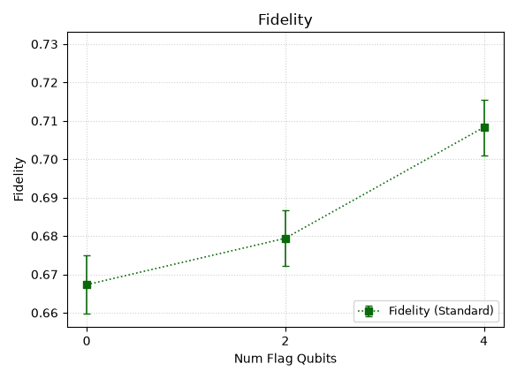
- \(19\) random angles instead of the blind scan's \(2N = 100\): \(5\times\) fewer circuits; \(1000\) shots per circuit (cost-limited), hence the wide error bars.
- Fidelity rises as flags are added: \(0.667 \to 0.708\) with \(4\) flags.
- More flags cover more of the tree, but each adds gates and costs acceptance, so we stopped at \(4\).
Run it yourself: metriq-gym
{
  "benchmark_name": "GHZ",
  "num_qubits": 26,
  "method":
    "compressed_sensing",
  "num_phases": 20,
  "shots": 30000
}
- One dispatch, one poll, on any supported backend (IBM, Quantinuum, IonQ, local simulators); the estimator and the \(n_{\mathrm{rec}} = N\) size check come built in.
- DFE and full parity oscillation are included as alternative verification methods for comparison.
Thanks!
Vincent Russo
vprusso.github.io
vincentrusso1@gmail.com
github.com/vprusso
Paper: arXiv:2604.27824
Blog: vprusso.github.io/posts/ghz_cs/
Unitary Foundation is hiring
unitary.foundation/jobs/mtscs